Chapter 14 Evaluating Predictions
14.1 Residuals
Not every prediction is going to be perfect. That’s actually built into the fabric of regression! What regression is really doing is predicting the average \(y\) for each value of \(x\). Have a quick look at the plot from the last chapter.
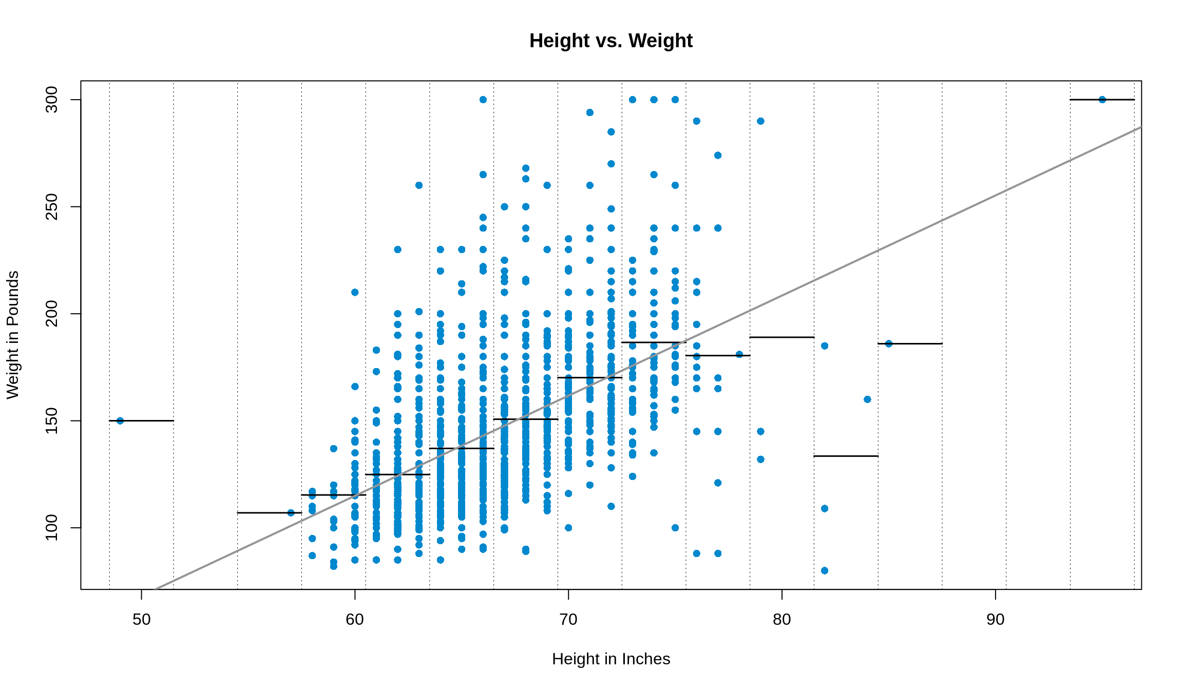
Each of the horizontal lines represents the average of the bin (defined by the dotted, vertical lines) and the regression line is plotted in grey. As you can see, the line predicts the average value for a group of data (for the majority of it, anyways).
However, obviously not every point is located right at that group’s average value. This means we’ll have some error in our prediction, called a residual. We calculate a residual to be the actual value minus the predicted value. Points that are above their predicted value (i.e. people that are heavier than we predict them to be) have positive residuals. Points that are below their predicted value have negative residuals. Points that fall on the line, or are exactly their predicted value, have no residual.
Under the hood, when we fit the regression line with lm(), R knows to try and minimize the residual value of each point. In fact, the line finds a way to make the residuals sum (and therefore average) to be 0.
14.2 Root Mean Squared Error (RMSE)
So, if the average of each \(x\) value is really what the regression line is predicting, there’s probably some spread around that prediction. Exactly right! The standard deviation of the prediction errors, or root mean squared error (RMSE) is what you’re thinking of.
Just like a standard deviation does with a normal curve, the RMSE lets us talk about a range of prediction errors and attach wiggle room to our predictions. To get the formula for this new RMSE thing, reverse the order of the words in the name. Start by finding the prediction error. That is, for each \(y\) value in our data (we’ll call it \(y_i\)), subtract off the predicted value. We called a prediction \(\hat{y}\) earlier, so we’ll call each individual prediction \(\hat{y}_i\) now.
\[ \text{Prediction Error} = \text{Actual} - \text{Predicted} = y_i - \hat{y}_i \]
Then, square each prediction error:
\[ \left( y_i - \hat{y}_i \right) ^ 2 \]
Take the mean of these squared errors. We’ll assume that there’s \(n\) predictions (read: observations) in our data.
\[ \frac{1}{n} \sum_{i = 1} ^ n \left( y_i - \hat{y}_i \right) ^ 2 \]
Finally, to get the RMSE, take the square root of this.
\[ \text{RMSE} = \sqrt{\frac{1}{n} \sum_{i = 1} ^ n \left( y_i - \hat{y}_i \right) ^ 2} \]
While this may seem daunting, this is one way to calculate the RMSE. It’s easy to remember as long as you read the name in reverse order. However, there’s another way to calculate the RMSE that we talk about in class.
\[ \text{RMSE} = \sqrt{1 - r ^ 2} \cdot \text{SD}_y \]
They should give us the same number, but do they? We’ll find the RMSE of the data we’ve been working with to check. Remember, we’re predicting weight from height in survey1, so weight is our \(y\) variable. We’ll make use of R’s vectorization again to do our calculations. Make sure that you pay attention to where the parentheses go!
## [1] 28.14292## [1] 28.14292Pam, your thoughts?

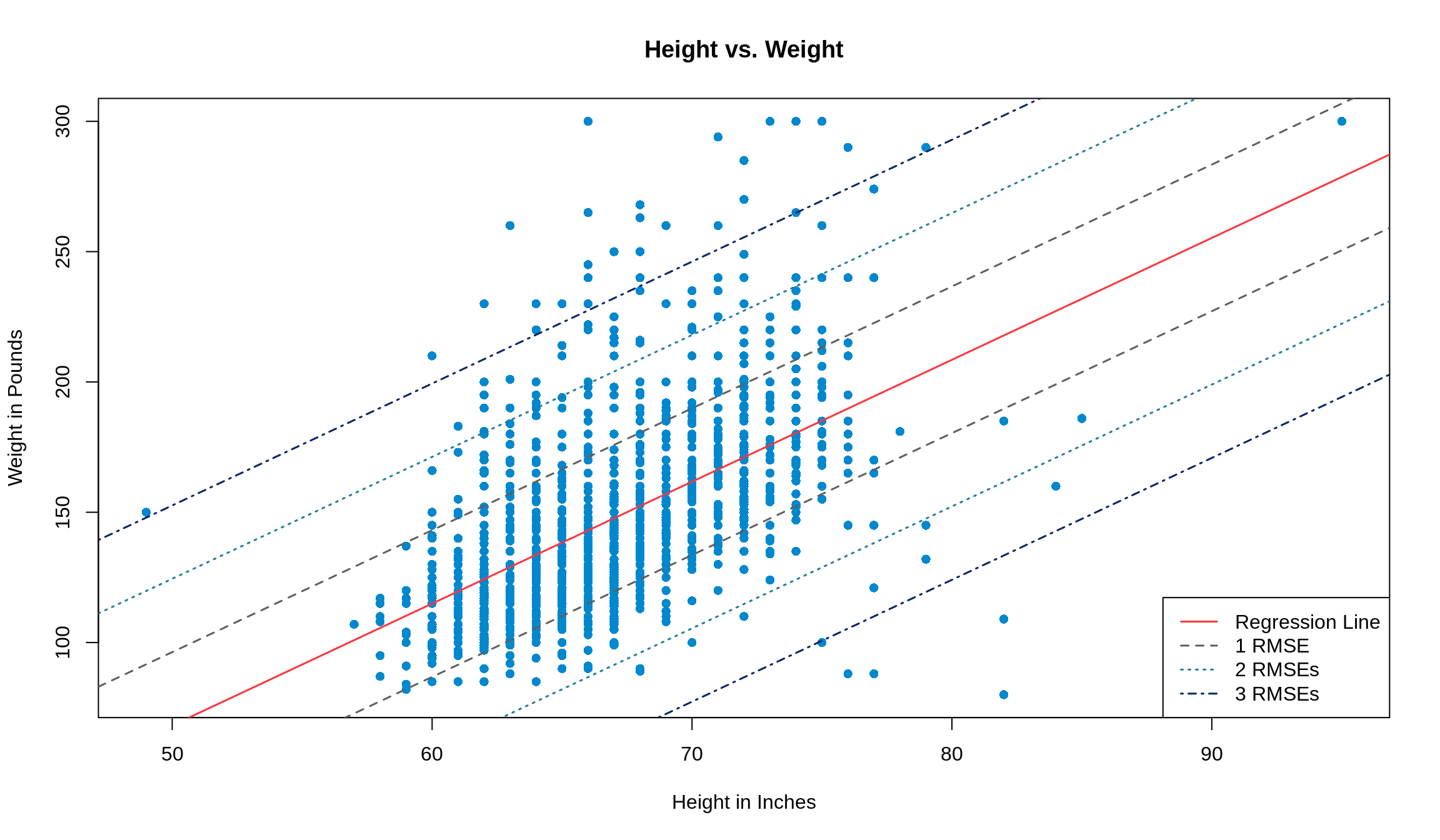
The same rules apply to the RMSE that applied to standard deviations. 68% of our data will fall within 1 RMSE of its predicted value, 95% will fall within 2 RMSEs of its predicted value, and 99% will fall within 3 RMSEs of what we predict. To see it graphically, look no further.